How to Find Duplicates in Excel: Highlight, Filter, Review

You've just merged 1,000 customer records and found duplicates. Deleting them immediately can create problems that are difficult to undo.

When working with critical data like customer lists, transaction records, or inventory, you need to identify and review duplicates before deciding what to remove.

This guide shows you how to find duplicates in Excel by highlighting them with conditional formatting and filtering duplicate rows step by step.

When You Need to Find Duplicates in Excel

Finding duplicates in Excel is different from removing them. Before cleaning your data, you need to understand where duplicates exist and how many there are to work safely without mistakes.

For example, if the same email appears multiple times in a signup list, you need to keep the most recent information and delete the rest.

By using conditional formatting to highlight duplicates and Excel filters to extract them, you can review duplicate patterns clearly before taking action.

Combining conditional formatting and filters lets you manage duplicate data without using complex formulas.

1. Highlight Duplicates in Excel with Conditional Formatting

Using Excel's conditional formatting feature with cell highlighting rules can be done quickly to highlight duplicates.

Select Range and Apply Conditional Formatting for Duplicates

1. Click the first cell of the data range you want to check for duplicates. For example, if email addresses are in column B, select cell B2.
2. Press Ctrl+Shift+Down Arrow to select all the way to the end of your data. This shortcut lets you quickly select large datasets.
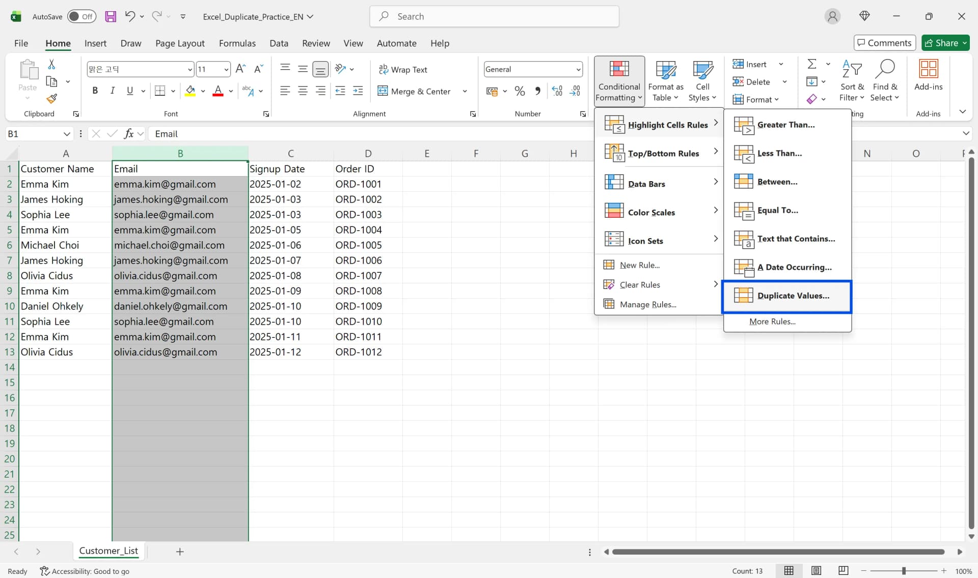
3. Click Conditional Formatting in the Home tab.
4. Select Duplicate Values from the Highlight Cells Rules menu.
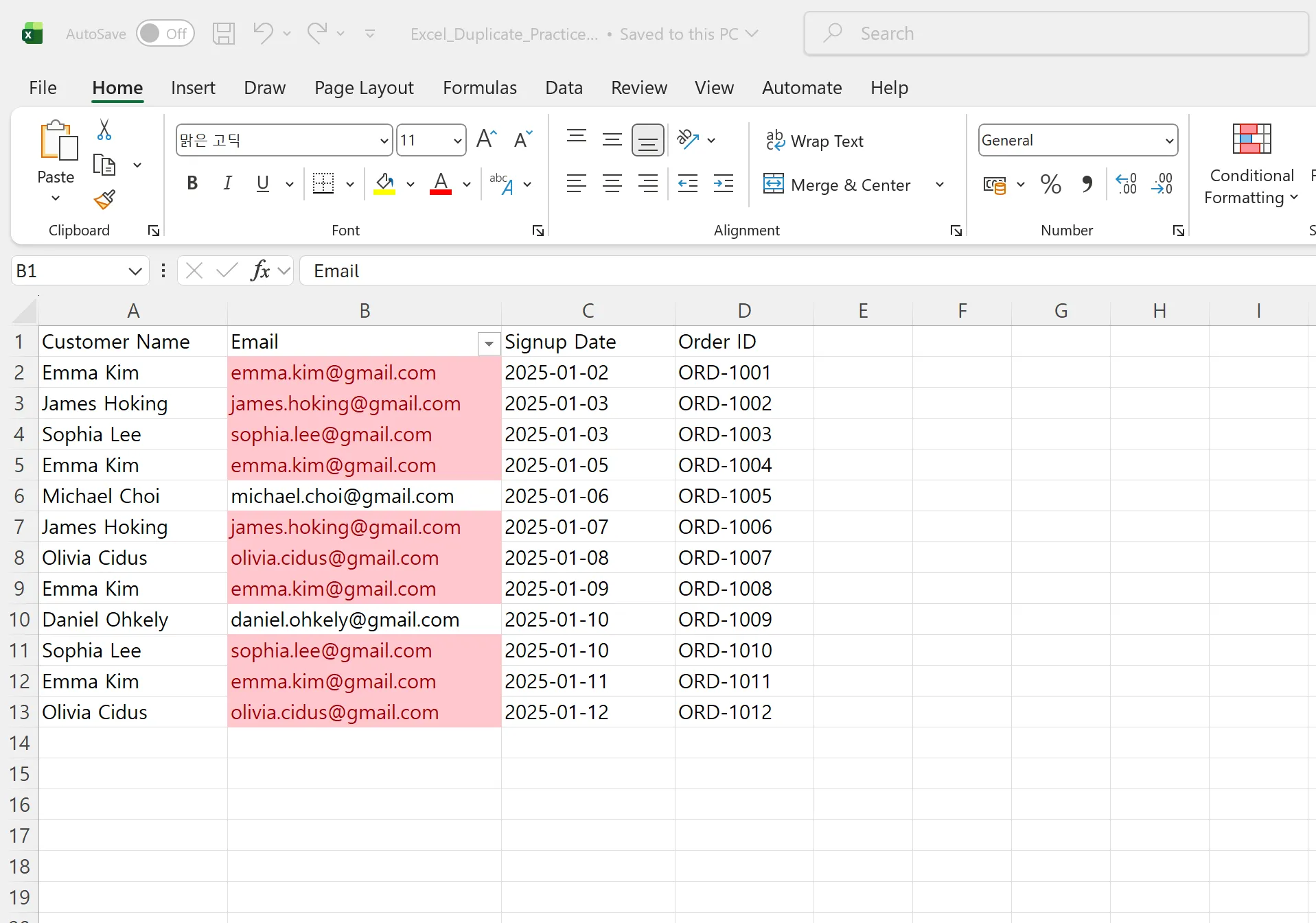
5. When the Duplicate Values dialog appears, confirm that the first dropdown shows "Duplicate."
6. Choose your desired color from the format dropdown. By default, it offers light red fill with dark red text.
7. Click OK, and duplicate values will be highlighted in your chosen color.

Customize Conditional Formatting to Highlight Duplicates

1. In the Duplicate Values dialog, click Custom Format instead of the format dropdown.
2. When the Format Cells dialog opens, choose from the Font, Border, or Fill tabs.
3. In the Font tab, click the Color option and select your preferred color. You can change from Automatic (black) to blue, green, or any other color.
4. In the Fill tab, click your desired color to set the background.
5. Click OK twice to apply your custom formatting and complete highlighting duplicates in Excel.

2. Highlight Duplicates in Excel Using COUNTIF

While the basic conditional formatting duplicates Excel rule is simple, using the COUNTIF formula directly gives you more control when you need to find duplicate rows Excel that meet specific conditions.

Highlight All Duplicate Items in Excel with COUNTIF

1. Assume your data exists from B2 to B100. Drag to select the entire range.
2. Click Conditional Formatting in the Home tab.
3. Select New Rule.
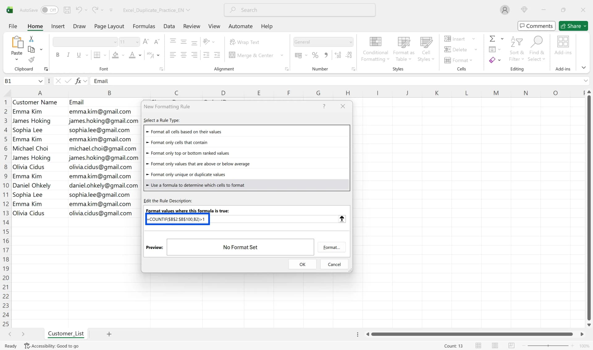
4. Click "Use a formula to determine which cells to format."
5. Enter =COUNTIF($B$2:$B$100,B2)>1 in the formula field.
6. Click the Format button to specify your desired color, then click OK.
7. Click OK again, and all values appearing 2 or more times in the range will be highlighted.

Highlight Only Second and Later Duplicates

1. Select the data range and click Conditional Formatting > New Rule.
2. Choose "Use a formula to determine which cells to format."
3. Enter =COUNTIF($B$2:B2,B2)>1 in the formula field. Notice the ending range (B2) has no dollar signs.
4. Set your color in the Format button and click OK twice.
5. The first occurrence won't be highlighted, only second and later duplicates will be colored.

Find Duplicate Rows in Excel Based on Multiple Columns

1. If you have names in column A and dates in column B, and want to find duplicate rows Excel where both values match, select the A2:B100 range.
2. Go to Conditional Formatting > New Rule > "Use a formula to determine which cells to format."
3. Enter =COUNTIFS($A$2:$A$100,$A2,$B$2:$B$100,$B2)>1 in the formula field.
4. Set your color in the Format button and click OK twice.
5. All rows where the name and date combination repeats will be formatted, completing your formula-based duplicate detection.

3. Find Duplicate Rows in Excel Using Filters

Once you've used Excel's conditional formatting to highlight duplicates, you can use Excel filters to show only duplicate rows and hide the rest.

Apply Filter to Find Duplicate Rows Excel by Color

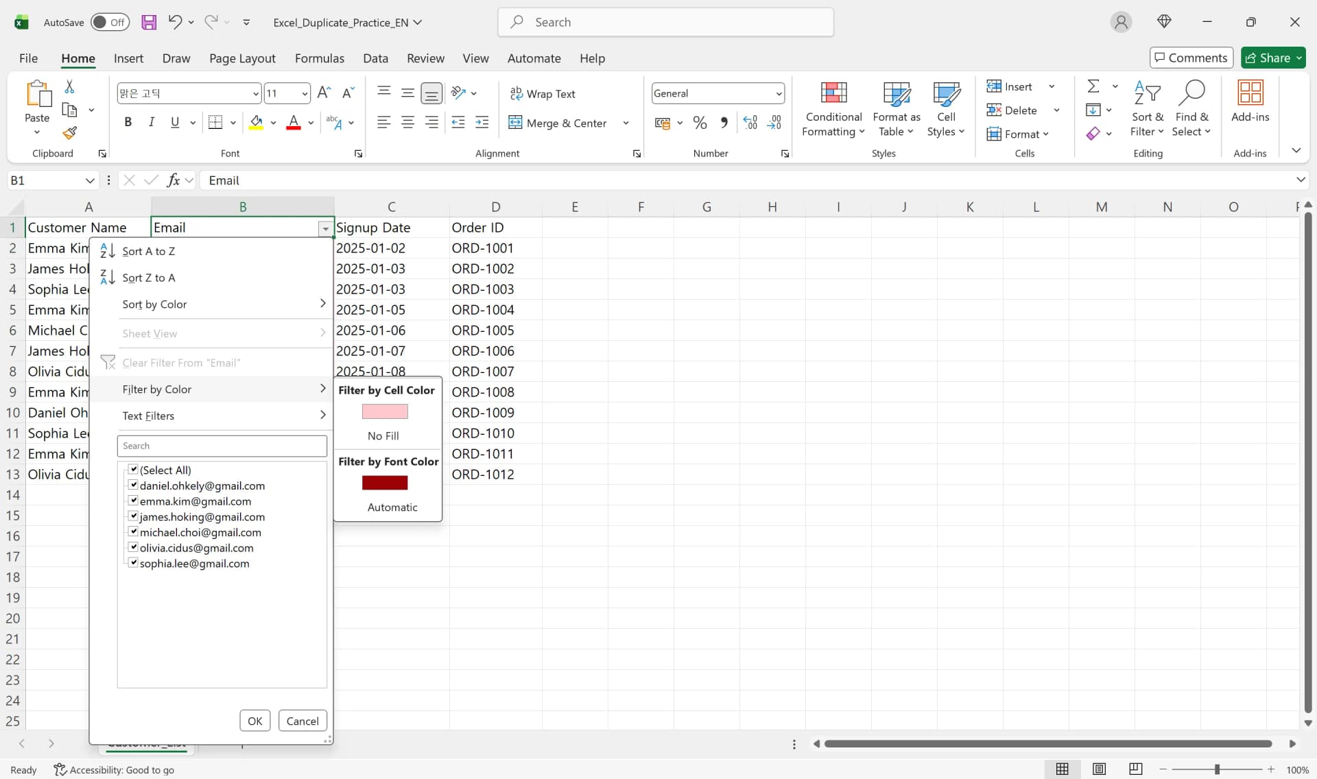
1. Click Filter in the Data tab. Filter arrows will appear in your header row.
2. Click the filter arrow in the column with duplicate highlighting.
3. Select Filter by Color from the menu.
4. Click the fill color or font color you used in conditional formatting.
5. Only rows with that color (i.e., duplicate rows) will be displayed on screen.
6. To remove the filter, click Filter again in the Data tab to return to your full dataset.

Group Duplicate Rows with Sorting

1. With duplicates colored, click the filter arrow in that column.
2. Select Sort A to Z or Sort Smallest to Largest.
3. Identical values will group together consecutively, making deletion or copying much easier.
4. Combining color filtering and sorting lets you review duplicate entries more efficiently.

Practical Tips for Finding Duplicates

When learning how to find duplicates in Excel, following a few precautions can prevent mistakes. It is recommended to work on a copy of the original sheet before making changes. Since identifying and deleting duplicates risks data corruption, work on a copy first, verify results, then apply to the original.

Convert your data range to a table using Ctrl+T to automatically enable filtering and sorting, and conditional formatting will auto-expand when you add new rows. Using the table feature means you don't need to reselect ranges manually—rules apply automatically as data grows.

When using COUNTIF or COUNTIFS functions to highlight duplicates with conditional formatting, you must distinguish between absolute and relative references correctly. Typically, set the first argument as an absolute reference ($B$2:$B$100) to lock the entire range, while the second argument should be a relative reference (B2) so the comparison target changes for each row. Learning this pattern makes formula-based duplicate detection much easier.

How to Find Duplicates in Excel - Frequently Asked Questions

Q. What's the difference between finding and removing duplicates in Excel?

Finding duplicates only highlights where duplicates exist without deleting data. After using conditional formatting or filters to review duplicates, you can decide which items to keep or remove. In contrast, the Remove Duplicates feature in the Data tab deletes immediately and is difficult to recover.

Q. Why use absolute references in COUNTIF when highlighting duplicates in Excel?

Conditional formatting applies formulas repeatedly to each row. Without absolute references (B$2:B$100), the comparison range shifts as rows change, producing incorrect results. Keep the comparison target as a relative reference (B2) while locking the entire range with absolute references for accuracy.

Q. Can I delete duplicates highlighted by conditional formatting all at once?

Conditional formatting only highlights—it doesn't have a delete function. Apply a color filter to display only duplicates, then manually select and delete rows or use the Remove Duplicates feature in the Data tab.

Q. How do I find duplicate rows Excel based on multiple columns?

Use the COUNTIFS function. For example, the formula =COUNTIFS($A$2:$A$100,$A2,$B$2:$B$100,$B2)>1 identifies rows where both column A and column B values match.