Blog
Freeze Top Row and Columns in Excel While Scrolling
 Mike Yi · Dec 26, 2025
Monday morning, and you're organizing 100 rows of sales data for your manager.
As you scroll down to check amounts, you lose track of what each column means. Scrolling back up to see the header, then down again. It wastes time.
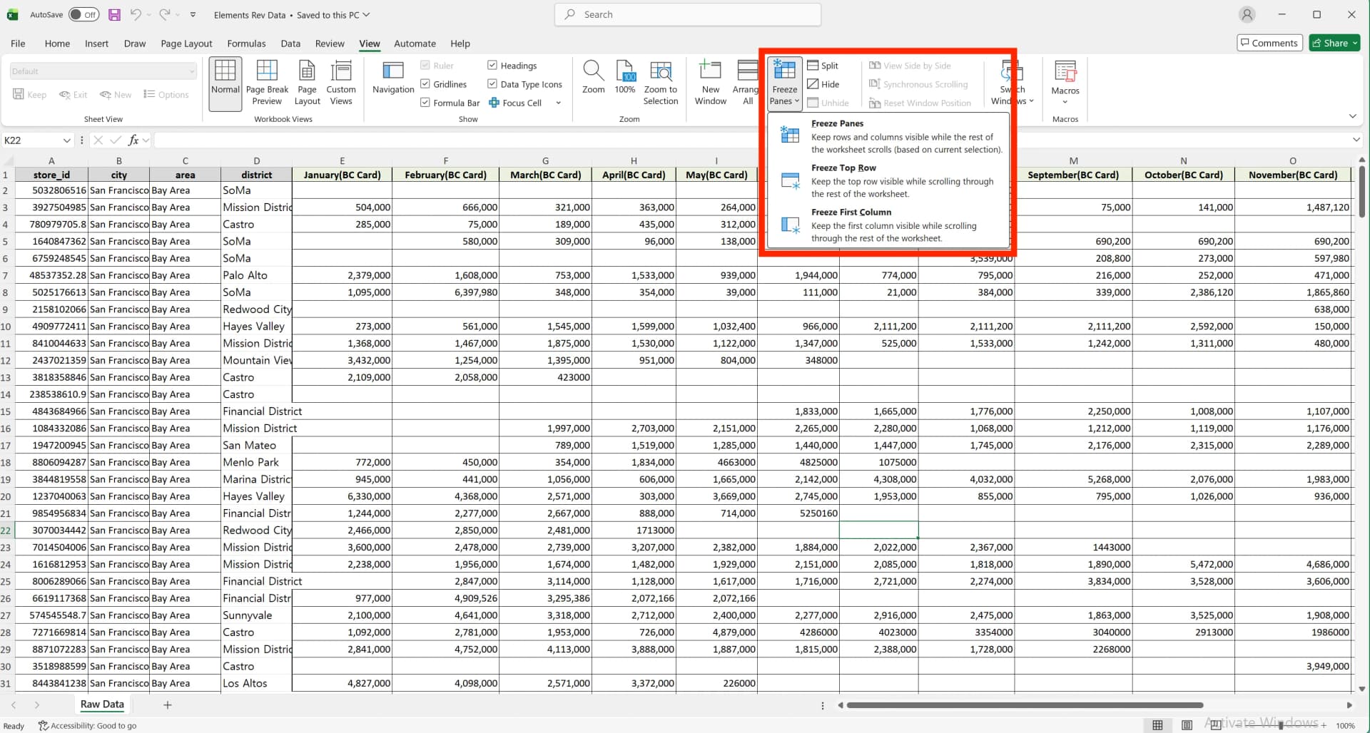
Excel's freeze panes feature solves this. Keep your header row visible while scrolling, so you can review data faster and work more efficiently. This guide covers how to Freeze Top Row in Excel, plus solutions to common issues.

Freeze Top Row vs Freeze Panes in Excel: What's the Difference?
These features sound similar, but they work differently.
Freeze Top Row locks only the first row at the top of your screen. Your header row stays visible when you scroll down. This is perfect for data tables.
Freeze Panes locks both rows and columns. Your header row stays visible when scrolling down, and your left column stays fixed when scrolling right. For example, freeze the employee name column and header row together. Now you always know whose data you're looking at, no matter where you scroll.
Quick summary:
To freeze only rows, use Freeze Top Row. To freeze both rows and columns, use Freeze Panes.
Both options are in View > Freeze Panes.
Freeze Top Row vs Freeze Columns vs Freeze Panes
| Category | What stays visible | Best for | Where to click |
|---|---|---|---|
| Row | Top Row | Header rows | View > Freeze Panes > Freeze Top Row |
| Column | First column | Names/IDs | Freeze Panes > Freeze First Column |
| Panes | Rows + columns | Large tables | Select a cell, then View > Freeze Panes > Freeze Panes |
How to Freeze Top Row in Excel
Freeze the First Row Only
This is the simplest method. Use it when you only need to freeze your header row.
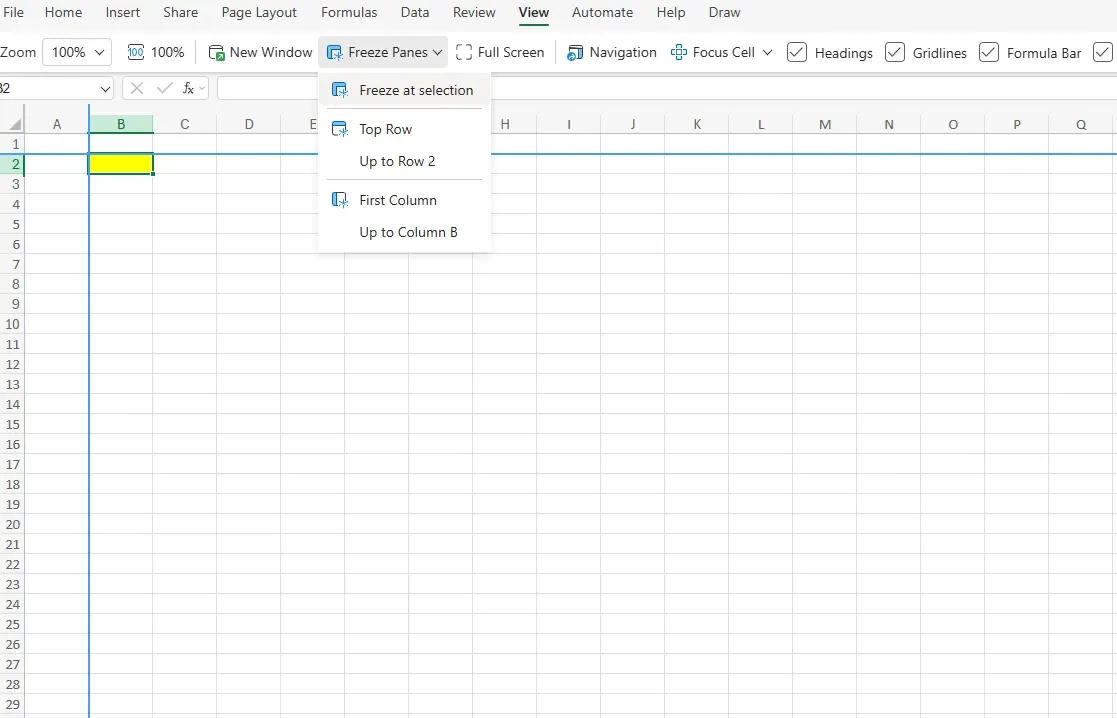
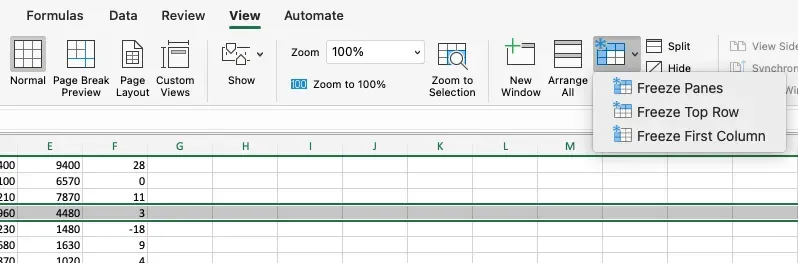
- Go to View tab
- Click Freeze Panes > Freeze Top Row
Now your first row stays at the top when you scroll down.
You'll see a thin gray line below the frozen row.
Freeze Multiple Rows
Need to freeze more than one row? Use this when you have multi-level headers (like main categories in row 1 and subcategories in row 2).
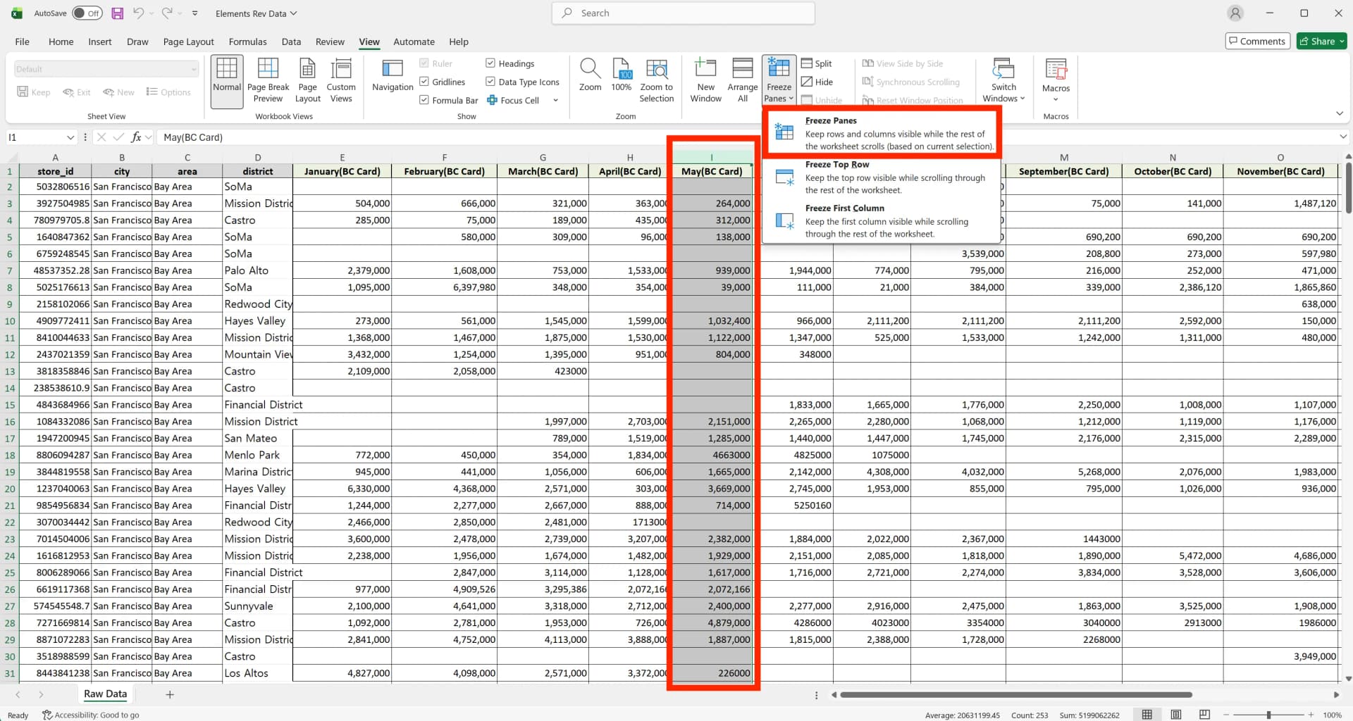
- Click the row number below the rows you want to freeze (e.g. click row 3 to freeze rows 1–2).
- Go to View > Freeze Panes > Freeze Panes
All rows above your selection will be frozen. For example, selecting row 3 freezes rows 1-2, while selecting row 5 freezes rows 1-4.
Freeze the First Column
Need to freeze a column instead? This works great for columns you always need to see, like employee names or product codes.
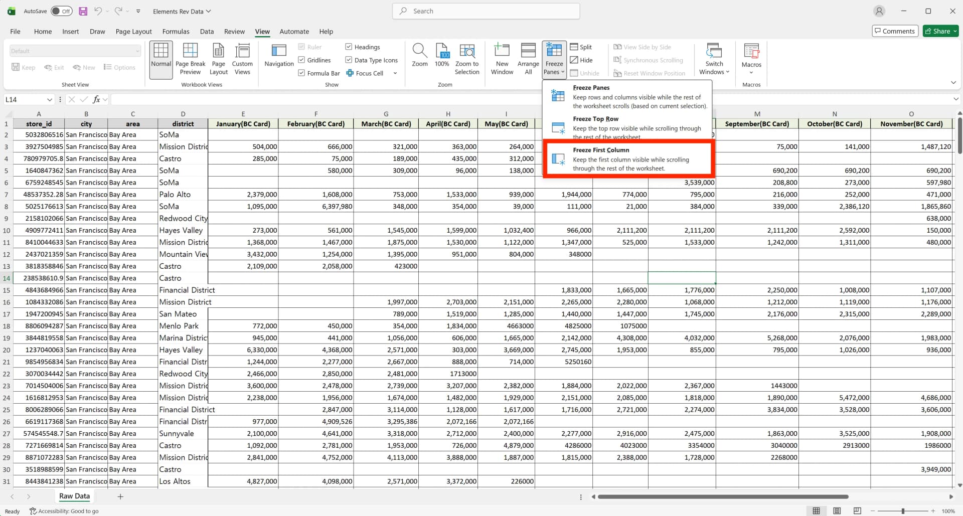
- Go to View > Freeze Panes
- Click Freeze First Column
Now column A stays on the left when you scroll right.
How to Freeze Top Row and Columns Together
This is the most useful method for large datasets—freeze both your header row and left column at the same time.
How Freeze Panes Works
The key is selecting the right cell. Click the cell diagonally below and to the right of what you want to freeze.
Examples:
- Freeze row 1 + column A = select cell B2
- Freeze row 2 + column B = select cell C3
Steps to Freeze Top Row and Columns
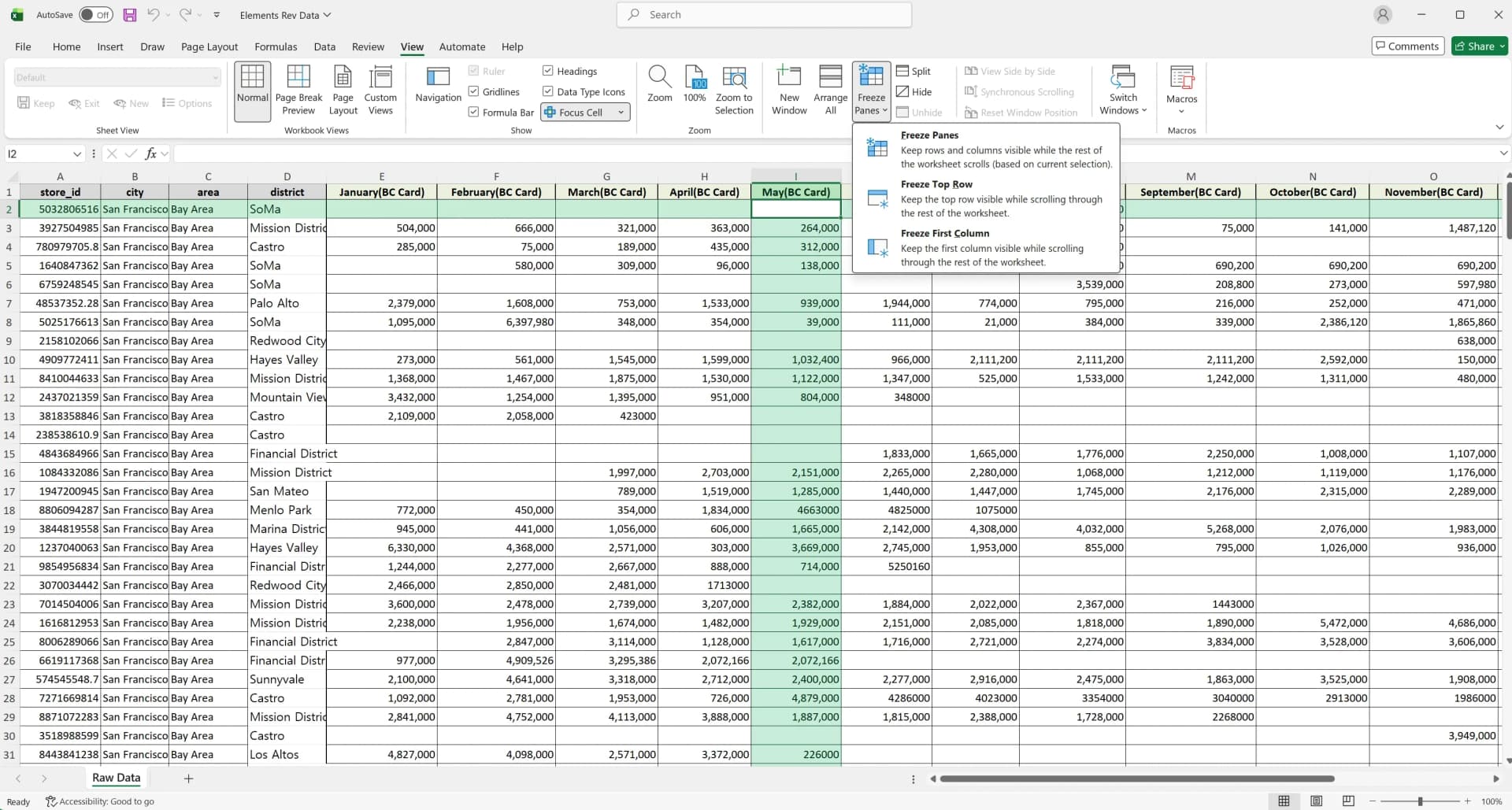
- Click the cell below your target row and to the right of your target column
- Go to View > Freeze Panes > Freeze Panes
Now your header row stays visible when scrolling down, and your left column stays visible when scrolling right. Your key data is always on screen, no matter where you scroll.
Check Your Frozen Area
Look for gray lines. They show what's frozen.
A horizontal line = frozen rows.
A vertical line = frozen columns.
Both lines (cross shape) = both frozen.
Troubleshooting: Common Freeze Panes Issues
Q. Why does my freeze keep turning off when I scroll?
Solution: If Freeze Panes doesn't seem to be working, the sheet may already have an existing freeze setting, or you may be freezing the wrong row/cell selection. In some cases, filters and Excel Tables can make the freeze line hard to notice visually.
If the freeze line looks off after applying filters, try this:
- Go to View > Unfreeze Panes
- Confirm which cell to select for the freeze you want
- Apply Freeze Panes again
- Reapply filters if needed
Q. Can I freeze multiple areas in one sheet?
No. Excel allows only one freeze setting per worksheet, so you can’t freeze the top header and a bottom total row at the same time.
If you need a workaround, you can split content across multiple worksheets and freeze different areas in each. Another option is using Split under View > Split, which creates separate scrolling panes instead of locking rows. For print-only needs, setting print titles separately may be enough.
Print with Frozen Rows: Repeat Headers on Every Page
Freeze panes only works on screen. For printing, set up print titles separately to repeat your header on every page.
How to Set Print Titles
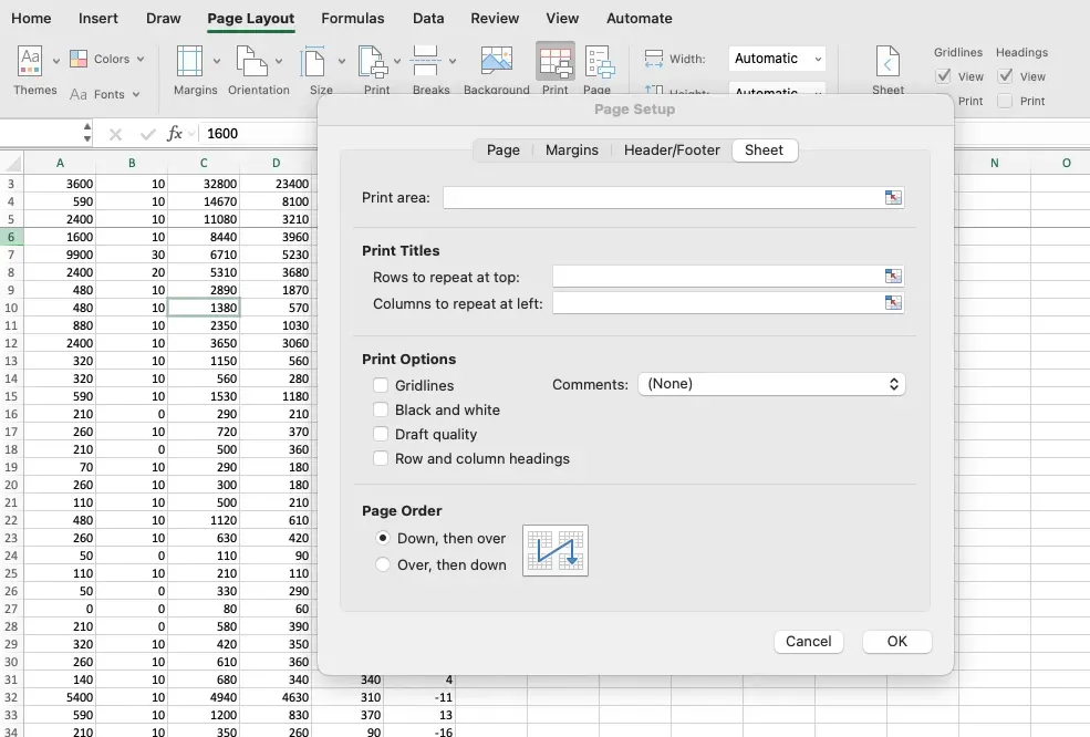
- Go to Page Layout > Print Titles
- In the Page Setup dialog, click Sheet tab
- Click the arrow next to "Rows to repeat at top"
- Select your header rows (e.g., type 1:2 for rows 1-2)
- Click OK
Check print preview. Your header now appears on every page, so you always know what you're looking at.
Freeze Panes Keyboard Shortcuts
Keyboard shortcuts are faster than clicking through menus.
It feels complex at first, but you'll memorize it quickly. If you use Excel daily, this shortcut alone will save you time.
Excel Row Freezing Shortcut Keys for Windows
Alt + W + F + F
Press these keys in order to freeze panes. Here's what happens:
- Alt shows shortcut keys on the ribbon
- W opens View tab
- F opens Freeze Panes menu
- F again selects Freeze Panes
How to Freeze Top Row in Excel on Mac
Using Excel on Mac? The process is the same as Windows, but menus are slightly different.
Steps for Mac
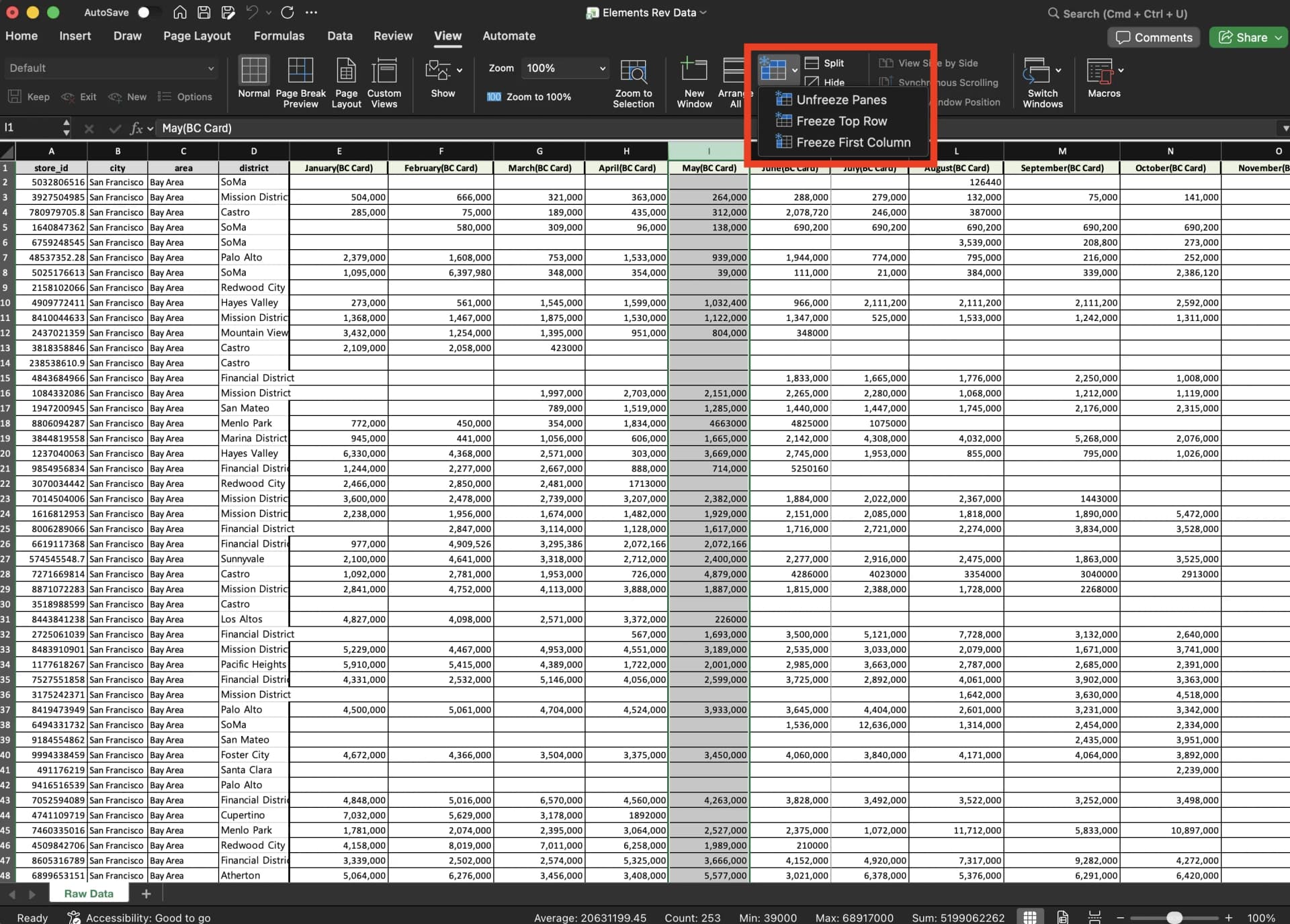
- Click the row below where you want to freeze (or column to the right)
- Go to View > Freeze Panes
Excel on Mac has the same Freeze Top Row and Freeze First Column options. The interface is nearly identical to Windows, so all methods above work the same way.
MacBook Excel Row Freezing Shortcut Key
Mac doesn't have a built-in freeze shortcut. Use View > Freeze Panes from the menu.
How to Unfreeze on Mac
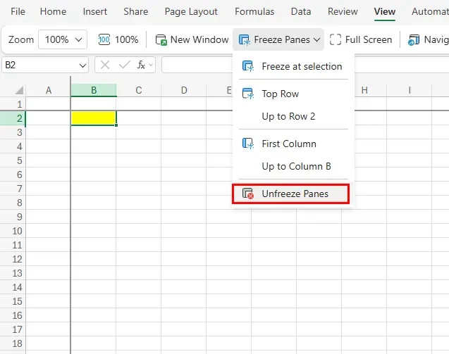
When you're done or want to view data differently, you can unfreeze the panes.
- Go to View > Freeze Panes
- If panes are frozen, you'll see Unfreeze Panes
- Click it
The gray line disappears and you're back to normal scrolling.
Best Practices for Freeze Panes
Here's what works best in real-world use.
- For very complex sheets (merged cells, grouped rows, heavy tables), freezing both rows and columns can feel cluttered. Try freezing only what you need.
- Freeze before filtering. Always set freeze panes first, then add filters. This prevents scrolling issues.
- Keep it simple for complex tables. For complex tables, freeze either rows or columns, not both. Freezing both can cause display issues with merged cells or grouped rows.
- Save as template. Create a template with freeze panes already set. You won't need to reconfigure it each time.
Stop Manually Freezing Rows. Start Automating Your Entire Excel Workflow.
You've learned how to freeze panes manually. But what if you could automate the repetitive Excel work that comes after?
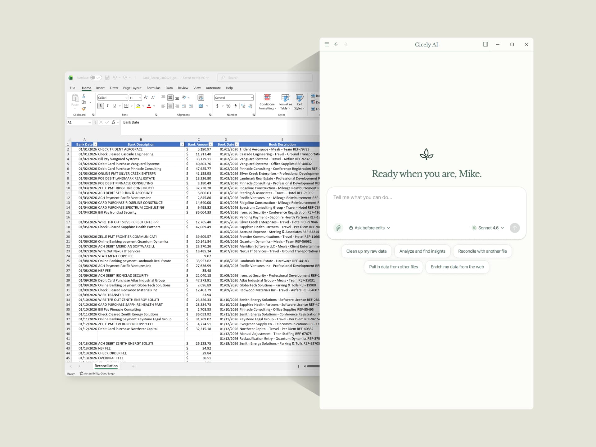
Cicely AI is a desktop-native AI coworker built specifically for Excel. Instead of manually formatting tables, cleaning messy data, and merging files one by one, Cicely works directly inside your Excel workbooks on your computer.
Unlike ChatGPT or web-based tools, Cicely doesn't require uploading or copy-pasting. Tell Cicely what you need in plain English. "Merge these 50 sales files into one table," "Remove duplicates and format as currency," or "Cross-reference customer data from this PDF." Cicely scans your local files, consolidates the data, and delivers analysis-ready spreadsheets while you review each change.
Everything runs locally on your PC. No file uploads. No browser tools.