Freeze Top Row and Columns in Excel

When working with data in Excel, you’ve probably experienced this situation more than once: as soon as you scroll down, the most important column headers or reference rows disappear from the screen, forcing you to scroll back up just to check what each value means.

At first, this may feel like a minor inconvenience. But when it happens repeatedly, it significantly slows down your workflow and breaks your concentration.

This problem becomes even more noticeable when working with large spreadsheets such as transaction records, customer lists, or survey results—files with many rows and columns. Each time you compare or enter data, you end up scrolling vertically and horizontally, wondering, “What column does this number belong to?”

This is where Freezing Rows and Columns in Excel, also known as Freeze Panes, becomes extremely useful.

By using Freeze Panes, you can lock specific rows or columns in place so they remain visible while you scroll. This allows you to review and work with data much faster and more accurately.

In this guide, we’ll walk through how to freeze the top row in Excel, how to freeze columns, and how to freeze rows and columns at the same time. We’ll also explain how to unfreeze panes when you no longer need them, and how to fix common issues when Freeze Panes doesn’t work as expected, so you can apply these features confidently in real-world Excel tasks.

All explained step by step so you can apply them immediately in real-world work.

Why Freezing Rows and Columns in Excel Matters

By default, Excel scrolls the entire worksheet at once.

This isn’t an issue with small datasets, but as spreadsheets grow more complex, it quickly becomes inefficient.

For example:

• When the header row scrolls out of view, you have to remember what each column represents.
• When the first column disappears, you constantly need to scroll back to the left to check which row you’re looking at.

These repetitive actions not only waste time but also increase the risk of data entry errors and misinterpretation.

Using Freeze Rows and Freeze Columns allows you to keep key reference information visible at all times. In practice, Freeze Panes isn’t just a convenience—it’s an essential feature for improving both accuracy and speed when working in Excel.

How to Freeze Rows in Excel (Freeze Top Row)

Freezing the Top Row in Excel

The most commonly used option is Freeze Top Row. Since the first row usually contains column headers, it’s helpful to keep it visible while scrolling.

Here’s how to do it.

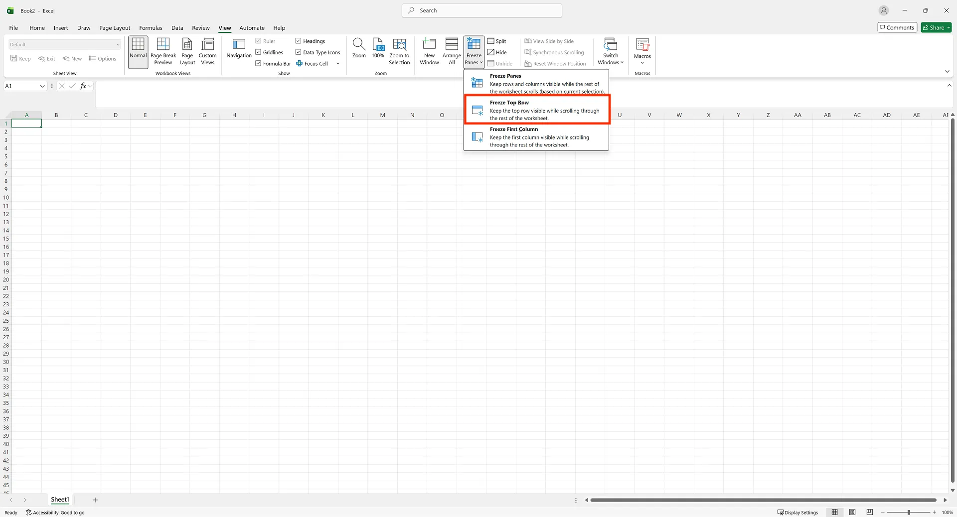
1. Click the View tab in the Excel ribbon.
2. Select Freeze Panes.
3. Click Freeze Top Row.

Once enabled, the first row will stay fixed at the top of the screen no matter how far you scroll down. The longer your dataset gets, the more valuable this feature becomes.

When Freezing the Top Row Is Especially Useful

• Transaction logs or sales reports that grow by date
• Survey results or customer data with repeated fields
• Reviewing data during meetings or presentations

Even freezing just the top row can dramatically improve how easily you understand and navigate your spreadsheet.

How to Freeze Columns in Excel

Freezing the First Column

Just like rows, freezing columns is also very common.

The first column often contains key identifiers such as names, IDs, or dates.

To freeze the first column

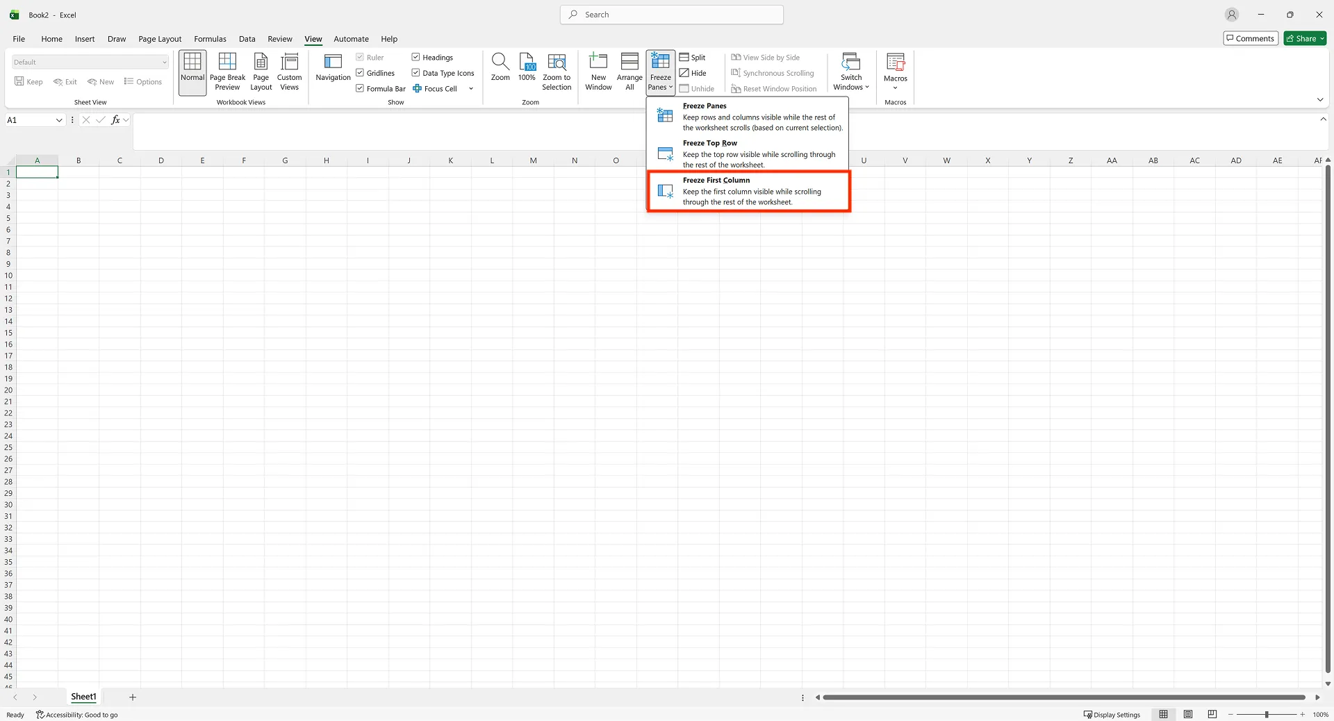
1. Click the View tab.
2. Select Freeze Panes.
3. Click Freeze First Column.

Now, when you scroll horizontally, the first column will remain visible on the left side of the screen. This is especially useful for wide spreadsheets.

How to Freeze Multiple Columns

If you want to freeze more than one column, it’s important to understand cell selection.

1. Select the cell immediately to the right of the last column you want to freeze.
2. Go to View → Freeze Panes → Freeze Panes.

All columns to the left of your selected cell will be frozen.

Without understanding this rule, it’s easy to feel confused about why the wrong columns are being frozen.

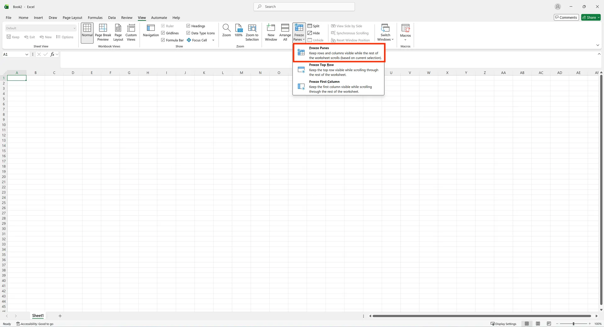
How to Freeze Rows and Columns at the Same Time (Freeze Panes Explained)

Understanding the Reference Cell

Excel allows you to freeze rows and columns simultaneously, but many users find this confusing because they don’t fully understand how Freeze Panes works.

Freeze Panes always freezes:

• All rows above the selected cell
• All columns to the left of the selected cell

For example, to freeze Row 1 and Column A, select cell B2, then apply Freeze Panes.

Once you understand this rule, you can control row and column freezing much more precisely.

Why Freeze Panes Sometimes Doesn’t Work as Expected

If you’ve ever thought, “Why didn’t this row freeze?” or “Why did the wrong column get frozen?” the issue is almost always the selected cell.

Before applying Freeze Panes, make it a habit to check that:

• The cell below the rows you want to freeze is selected
• The cell to the right of the columns you want to freeze is selected

How to Unfreeze Panes in Excel

Basic Way to Unfreeze Panes

To remove any frozen rows or columns

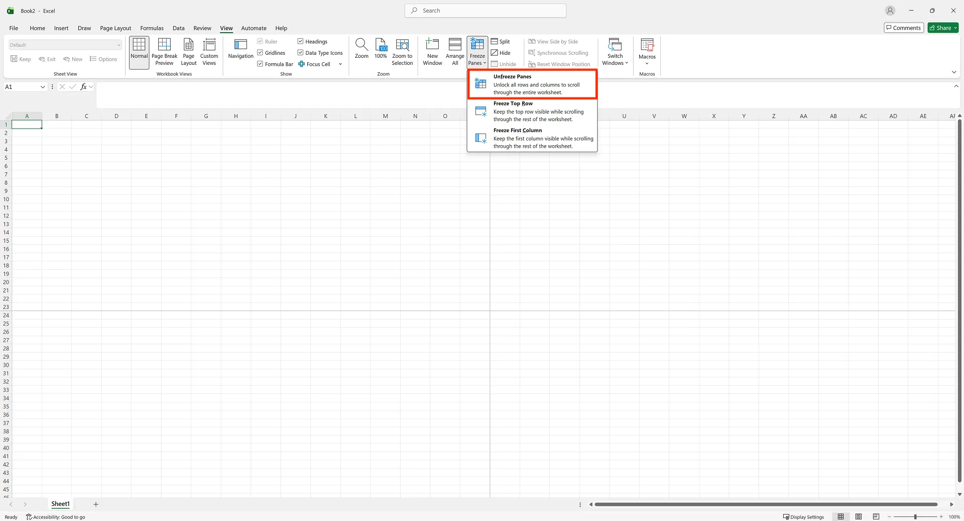
1. Click the View tab.
2. Select Freeze Panes → Unfreeze Panes.

This will remove all currently frozen rows and columns at once.

When It Looks Like Freeze Panes Didn’t Unfreeze

If the screen still looks strange after unfreezing, check the following:

1. Did you switch to another worksheet and back?
2. Is Split view turned on?
3. Did resizing the Excel window cause a visual illusion?

Split view is especially easy to confuse with Freeze Panes, so it’s worth checking.

When Freeze Panes Is Disabled in Excel

Why the Freeze Panes Option Is Grayed Out

Freeze Panes won’t work in the following situations.

• You are currently editing a cell
• The worksheet is protected

Exit cell edit mode, and if necessary, unprotect the sheet before trying again.

Top 3 Most Common Questions About Freezing Rows and Columns in Excel

Q1. Freeze Panes doesn’t work / the option is grayed out

A. This usually happens for one of two reasons:

1. You’re editing a cell → Press Enter or Esc to exit edit mode.
2. The sheet is protected → Unprotect the sheet from the Review tab.

Most issues are resolved by checking these two points.

Q2. The wrong rows or columns are frozen

A. Freeze Panes always freezes rows above and columns to the left of the selected cell.

For example, Freeze Row 1 and Column A → Select B2, then Freeze Panes and Freeze Rows 1–3 → Select a cell in Row 4, then Freeze Panes.

If something feels off, first check whether you selected the correct “next” cell.

Q3. What’s the difference between Freeze Panes and Split?

• Freeze Panes: Keeps specific rows or columns visible while scrolling
• Split: Divides the worksheet into multiple panes to view different areas at the same time

If you need to keep headers visible, use Freeze Panes.

If you want to compare distant parts of the same sheet, use Split.

One Rule to Remember About Freezing Rows and Columns

There’s one simple rule that solves most confusion:

“Select the cell immediately after the rows and columns you want to freeze, then apply Freeze Panes.”

Remembering this makes it easy to freeze rows, freeze columns, and unfreeze panes exactly the way you want.

Work More Efficiently in Excel with Cicely AI

Freezing rows and columns is just one step toward working efficiently in large spreadsheets. When setup and formatting tasks pile up, they take more time than the analysis itself.

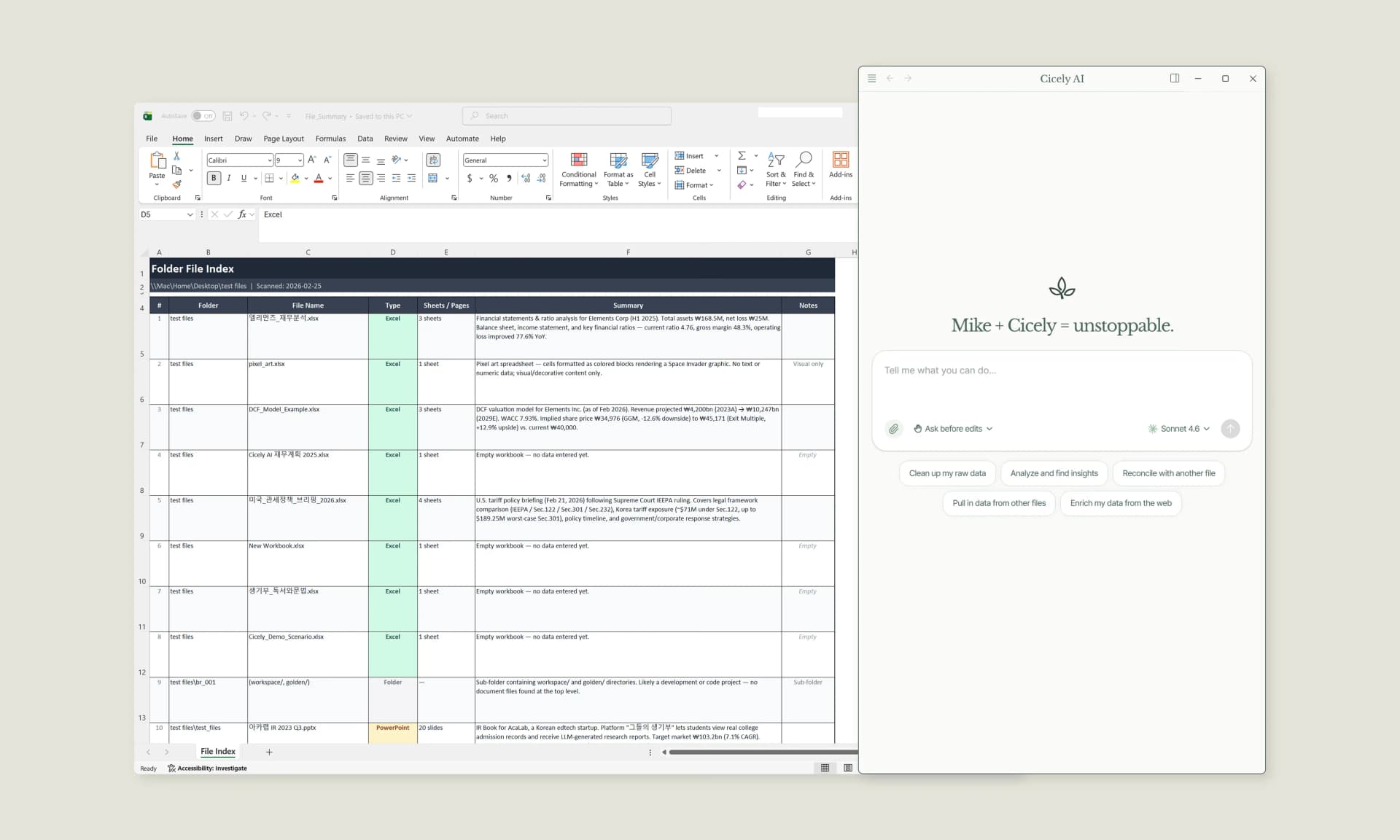
Cicely AI is a desktop-native AI coworker built for spreadsheet workflows. Instead of navigating menus manually, you can describe what you need in plain English, such as:

"Freeze the top two rows and first column on every sheet."

"Set up print titles so headers repeat on each page."

Cicely reviews your worksheet structure and guides you through the correct steps. Everything runs locally on your PC. No file uploads. No browser tools.